Nonlinear dynamics 1: Phase portrait
Sometimes chemical problems can be answered using knowledge of nonlinear dynamic analysis that is not directly related to chemistry. For example, some information about a complex reactions flow can be gained from the mathematical models of the interspecific competition. Oscillating chemical reactions such as the Bray-Liebhafsky reaction, the Briggs-Rauscher reaction , and the Belousov-Zhabotinski reaction provide wonderful examples of relaxation oscillations (nonlinear behavior) in science. They are often demonstrated in chemistry classes or used to astound the public at university open days. The first experiment of the BZ reaction was conducted by the Russian biochemist Boris Belousov in the 1950s, and the results were not confirmed until as late as 1968 by Zhabotinski (those examples will be addressed ina future post).
In this first post, we going to make a classic phase portrait analysis, considering non-isothermal CSTR problem, where we going to identify multiplicity steady-state. Due to the nonlinear behavior of chemical systems (strongly linked with the Arrhenius equation), the existence of multiplicity steady-state is often found when we are modelling or simulating a chemical system, sometimes we come across this behavior, experimentally.
Before we get started, let's define critical points (steady-state for engineering chemical accent) and how to classify them. First start with one of the simplest systems, a homogeneous linear system. Such a system has the form:
where \(\mathbf{A}\) is a matrix 2-by-2, and \(\mathbf{x}\) is a vector 2-by-1. From calculus we have solution family like \(\mathbf{x} = \mathbf{\omega} e^{\lambda t}\). So replace this into homogeneous system, we get:
with \(\lambda\) and \(\omega\) are the eigenvalue and eigenvector of \(\mathbf{A}\), respectively. In order to obtain the eigenvalue, we need to solve the characteristic equation (\(\mathrm{det}\left(\mathbf{A} - \lambda\mathbf{I} \right) = 0\)) and eigenvector from constraint \(\|\omega\| = 0\) and homogeneous system above.
The correspondent solution of the homogeneous linear system (i.e. when \(\mathbf{A}\mathbf{x}=0\)) is named by critical points and correspond to steady-states or equilibria of the system. The investigation of the critical point character, based on Lyapunov’s stability criteria, is closely related to the question of the system stability at the steady-state to small disturbances can be assessed first by linearization and then by computation of the eigenvalues of the Jacobian matrix:
Or qualitatively using phase portrait analysis. The phase portrait is a set of solving from a number of initial conditions, that will produce a phase path (a plot that shows the dependence of one unknown with the other) showing the behavior of the system along time integration. For example, given the linear system:
which has as critical point in the origin, and the eigenvalues of Jacobian: \(\mathbf{J} = \begin{bmatrix} a & 0 \\ b & b\end{bmatrix}\) are a and b. If \(a= -1; b=-5\) the phase portrait [1] looks like this:
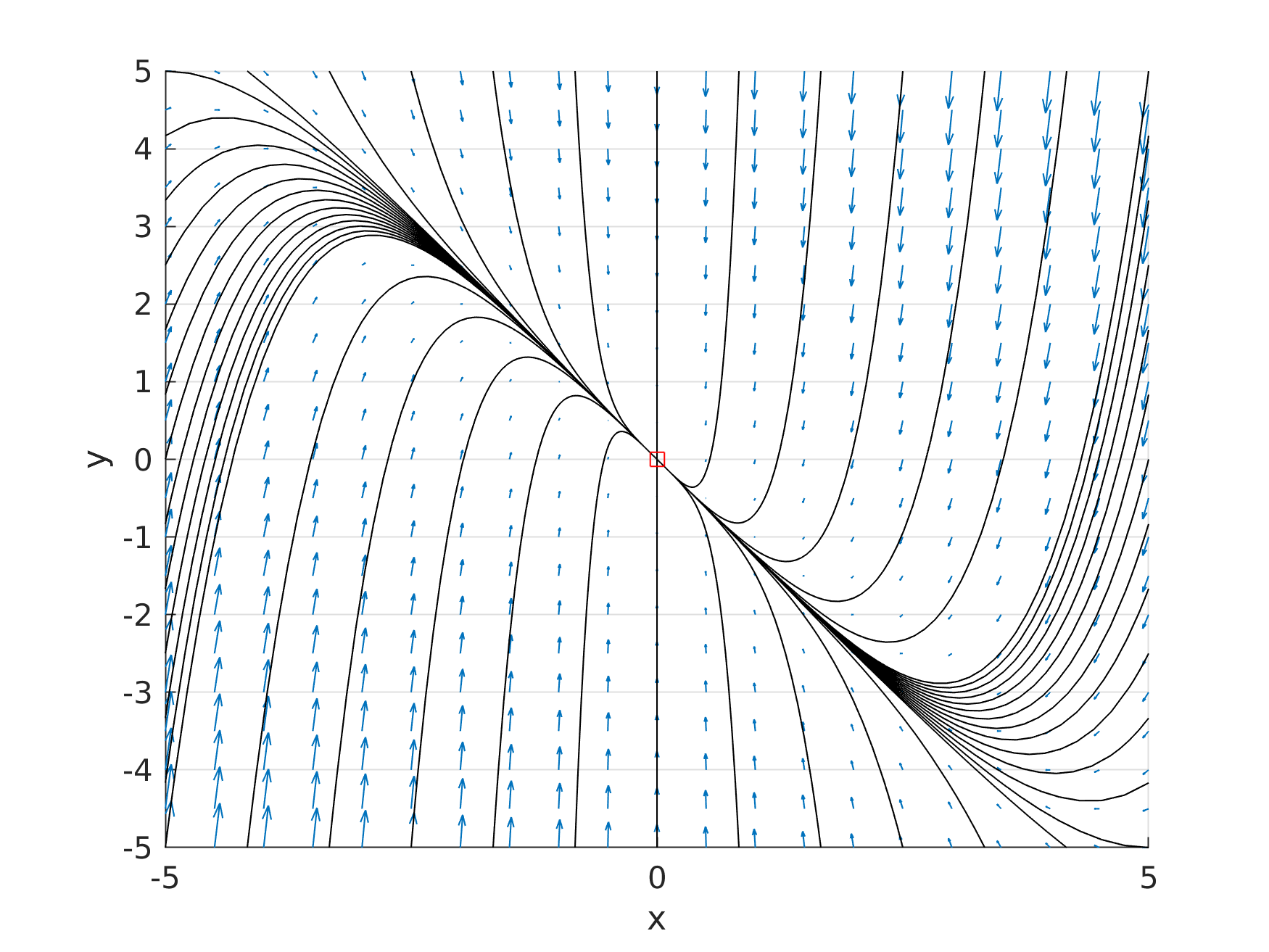
Phase portrait with a= -1 and b=-5.
Here all trajectories are lines through the origin (steady state of the system), this behavior is typically to attractor critical points. Others trajectories are ilustraited in Table below, with differents values for a and b:
Parameters values |
Phase portrait |
Critical point type |
|---|---|---|
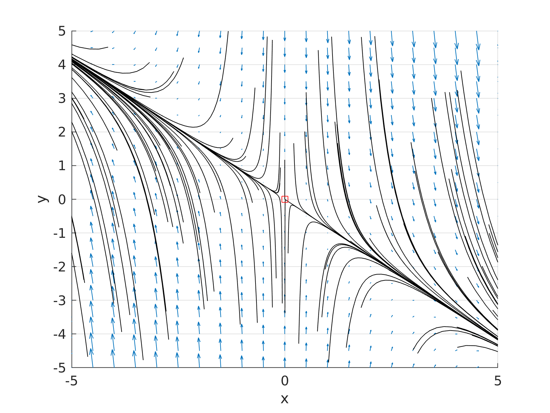
a = +1; b = -5 |
|
saddle point |
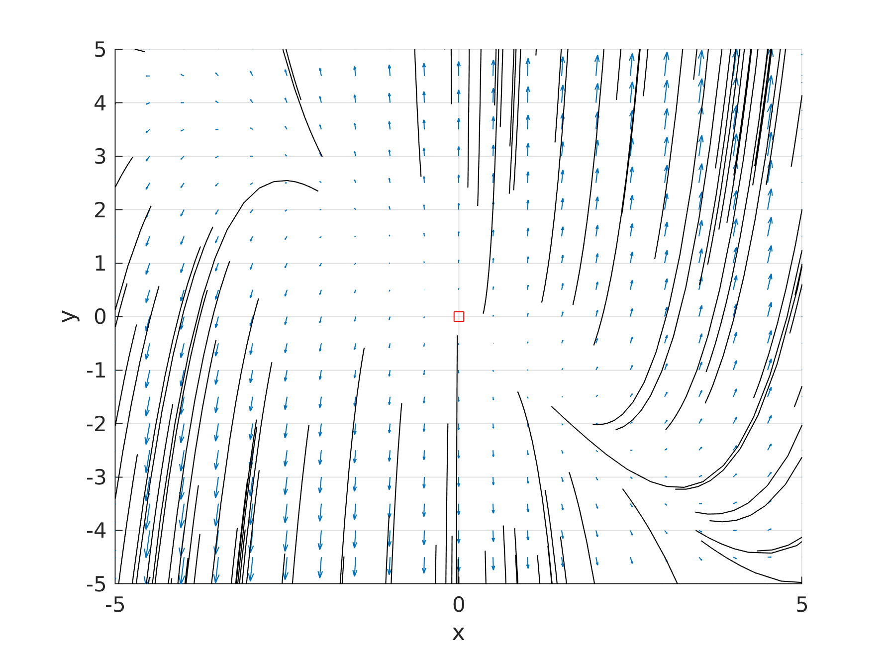
a = +1; b = +5 |
|
source point |
Those are commonly found in chemical reactors system, but there are others critical points types (center, spiral, star, degenerated,... more info, see the aforementioned references).
Here the chemical engineering kinetic borrows some terms from the dynamic system theory, without a deep discussion of the mathematical apparatus, we will show how the mathematical suites allow one to determine the critical point type. Assume the mathematical model of a process described by a set of two differential equations. As we saw above, in order to find the critical point type one has to: 1. Calculate the critical points (steady-states) on a phase plane, or solving the corresponding algebraic equation set (\(\mathbf{A}\mathbf{x}=0\)); 2. Compute the Jacobian matrix for the system using the critical points coordinates (\(\mathbf{J}(\mathbf{x0})\)); 3. Find the eigenvalues of the latter matrix, to establish the critical point type and the stability of the stationary state.
Non-isothermal reactor problem
Lets us consider the steady-state operation of a CSTR under non-isothermal conditions. If an exothermic reaction takes place in an isolated system (i.e. adiabatic reactor, absent of the heat exchange), a temperature will apparently increase over time, for example, hydrolysis of Propylene Glycol. The rate of this increase depends both on the kinetic parameters (rate constant) and on the thermodynamic properties of the system (thermal conditions of the reaction, heat capacity). For a well-mixed tank reactor, where a single first-order reaction: A + B → C occurs, the mathematical model is described by this set of equations:
where: \(\tau\) residence time, \(C_{Ao}\) the input reagent concentration, \(r_A = k_o e^{\frac{E}{RT}} C_A^n\) kinetic rate, \(T_o\) is the reagent temperature at entering reactor, \(\Delta H_{rx}\) heat of reaction, \(\rho|_{mx}\) misture density and \(C_p|_{mx}\) misture heat capacity. For simplicity, we assume that the heat capacity, heat reaction and density are temperature independent (i.e. constants) and the kinetic is a single first-order reaction. So, we can rewrite the model as:
with: \(G = \frac{\Delta H_{rx}}{\rho C_p |_{mx}}\).
Modeling the system of ODEs using the initial parameters:
\(G\) |
\(90.3\) |
\(\frac{E}{R}\) |
\(- 6307\) |
\(k_o\) |
17 x \(10^{+6}\) |
\(\tau\) |
60 |
\(C_{Ao}\) |
1.5 |
\(T_o\) |
250 |
We can find a stationary state through the phase portrait, from several initial conditions as ilustraited following:
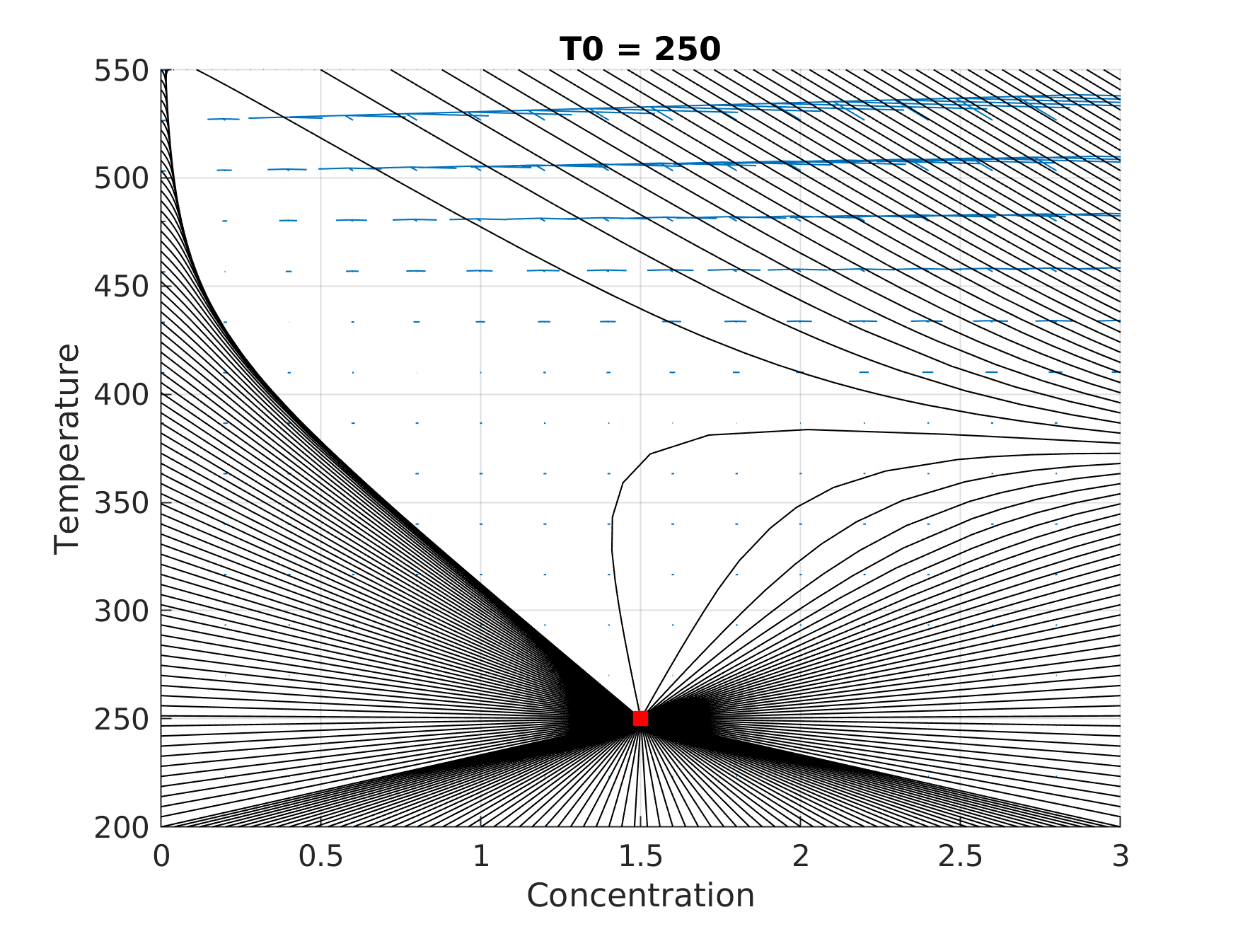
We can see that the steady-state (1.499, 250.015) is an attractor critical point, because all phase path toward it. The stationary state is linked to the thermal stability of the reactor (in the current case) and consequently with the convertion, that in this case is very slow. In order to confirm the attraction behavior, we analyze the Jacobian of the system using the critical point:
where we found the following eigenvalues: (-0.1667, -0.1666) < 0. The dynamic of this problem depends on the temperature of the initial mixture (as also: inlet concentration, residence time and etc), and thusas also the portrait can change strikingly. In the discussed example the steady-state is undesirable from the efficiency point of view. In order to enable the process, we need to increase the inlet temperature to improve the convertion and thus goes from old stationary to the other one, stable or may be unstable. If the latter one happens, any small perturbation of the system takes it out of the unstable state and goes to a stable one. Such situation is illustrated the animation below

When we change the input reagent temperature, we saw the presence of multiple steady-state (red square). In these cases (@ 322 and 331), the animation shows that two of the three possible stationary states are stable: for them the Jacobian matrix eigenvalues are real and of the same sign (stable point). The third steady-state has Jacobian eigenvalues real, but with signs opposite (saddle point).
\(T_o\) |
\(C_A, T\) |
eigenvalues of Jacobian \((C_A,T)\) |
|
|---|---|---|---|
@ 322.727 |
1.431, 328.90 |
-0.1670, -0.1140 |
Attractor |
0.736, 391.70 |
-0.1670, 0.0132 |
Saddle |
|
0.225, 437.80 |
-0.0478, -0.0167 |
Attractor |
|
@ 331.818 |
1.313, 348.70 |
-0.0167, -0.0044 |
Attractor |
1.110, 367.00 |
-0.0167, 0.0049 |
Saddle |
|
0.142, 454.50 |
-0.1141, -0.0167 |
Attractor |
This example by no means covers all possible problems of chemical reactor kinetics as well as other differential models for chemical-engineering processes, on which the nonlinear dynamic can be applied. In the next post, we'll be shown how to make a bifurcation diagram through software MatCont.